Decision Support Using Lighting-Corrected Intuitive Feature Models

Fig. 1

Workflow of the proposed melanoma decision support framework

Illumination Correction Preprocessing

Most illumination correction algorithms are not specific to skin lesion photographs and can be applied to any scene. Histogram equalization adjusts the distribution of pixel intensities, minimizing illumination variation globally [47]. Other algorithms correct for local illumination variation. These algorithms typically assume a multiplicative relationship between illumination and reflectance components. The estimated illumination component is estimated and used to find the reflectance component. The illumination component is assumed to be low-frequency, while the high-frequency detail is in the reflectance component. Using this assumption, there are many different algorithms that estimate illumination. One of the earliest is the Retinex algorithm, which uses a set of Gaussian filters of different sizes to remove detail and to estimate illumination [27, 36]. Morphological operators [49], bilateral filters [24], Monte Carlo sampling [53] and total variation [16] approaches have also been used to estimate illumination.

Other methods involve correction algorithms that are specific to images of skin lesions. Earlier algorithms enhance images taken with a dermatoscope to better separate lesion pixels from healthy skin. These algorithms include colour calibration [29] and normalization [33] to improve lesion classification or contrast enhancement [13, 46] to improve segmentation.

Recent work focuses on correcting photographs of skin lesions acquired using standard digital cameras to improve segmentation and classification. Work by Cavalcanti et al. [10] apply morphological operators to estimate the illumination component. The initial estimate of illumination is used to fit a parametric surface using the illumination intensities in the four corners of the photograph. The reflectance component is estimated using the parametric surface. Initial work on the correction algorithm outlined in this chapter was initially presented by Glaister et al. [28].

Feature Extraction and Classification

Most existing feature sets have been designed to model the ABCD criteria using dermoscopic images. Lee and Claridge propose irregularity indices to quantify the amount of border irregularity [37]. Aribisala and Claridge propose another border irregularity metric based on conditional entropy [6]. Celebi et al. propose shape, colour, and texture features with rationale, and using a filter feature selection method [12]. Colour features are primarily taken either in the RGB space (usually mean and standard deviation of the three channels), or a perceptually-uniform CIE colour space. Good overviews of existing features can be found in [35, 39].

Features designed to analyse dermoscopic images may not necessarily be suitable for the noisy unconstrained environment of standard camera images. Some work has been done to identify suitable features for standard camera images [1, 8, 9], however the focus of these methods has primarily been in the preprocessing and segmentation stages, resulting in large sets of low-level features. For example, Cavalcanti and Scharcanski [9] propose the same low-level feature set as Alcon et al. [1] with a few minor adjustments. Amelard et al. proposed the first set of high-level asymmetry and border irregularity features that were modeled assuming standard camera images [3, 4], which are used in this chapter.

Most of the methods use existing classification schemes, such as support vector machines (SVM), artificial neural networks (ANN), decision trees, and k-nearest neighbour (K-NN) [35]. Ballerini et al. designed a hierarchical classification system based on K-NN using texture and colour features to classify different types of non-melanoma skin lesions with 93 % malignant-versus-benign accuracy and 74 % inter-class accuracy [8]. Piatkowska et al. achieved 96 % classification accuracy using a multi-elitist particle swarm optimization method [44]. Thorough reviews of existing classification schemes can be found in [35, 39].

Some emphasis has been placed on constructing content-based image retrieval (CBIR) frameworks for recalling similar lesions. These methods rely on constructing a representative feature set that can be used to determine the similarity of two images. Ballerini et al. extracted basic colour and texture features such as colour mean, covariance, and texture co-occurrence matrix calculations, and used a weighted sum of Bhattacharyya distance and Euclidean distance to find visually similar lesions [7]. Celebi and Aslandogan incorporated a human response matrix based on psychovisual similarity experiments along with shape features to denote similarity [11]. Aldridge et al. designed CBIR software and experiments which showed with high statistical significance that diagnostic accuracy among laypeople and first-year dermatology students was drastically improved when using a CBIR system [2].

There has been some work done to extract melanin and hemoglobin information from skin images. The melanin and hemoglobin information can be very useful in trying to identify the stage and type of the lesion. All of the proposed methods rely on various physics-based models of the skin to characterize the reflectance under some assumptions about the absorption, reflectance, and transmission of the skin layers. Work primarily led by Claridge explores using multispectral images using spectrophotometric intracutaneous analysis to analyse melanin, hemoglobin, and collagen densities [19, 40]. Claridge used a physics-based forward parameter grid-search to determine the most feasible skin model parameters assuming standardized images [17]. Tsumura et al. used an independent component analysis (ICA) scheme to decompose the image into two independent channels, which they assumed are the melanin and hemoglobin channels [51]. D’Alessandro et al. used multispectral images obtained using a nevoscope and used a genetic algorithm to estimate melanin and blood volume [20]. Madooei et al. used blind-source separation techniques using a proposed corrected log-chromaticity 2-D colour space to obtain melanin and hemoglobin information [38].

Illumination Correction Preprocessing

The proposed framework first corrects for illumination variation using the multi-stage algorithm outlined in this section. The illumination correction algorithm uses three stages to estimate and correct for illumination variation. First, an initial non-parametric illumination model is estimated using a Monte Carlo sampling algorithm. Second, the final parametric illumination model is acquired using the initial model as a prior. Finally, the parametric model is applied to the reflectance map to correct for illumination variation. The three stages are outlined in this section.

Initial Non-parametric Illumination Modeling

The first stage involves estimating the initial non-parametric illumination model. This stage is required to estimate illumination robustly in the presence of artefacts, such as hair or prominent skin texture. Certain assumptions are made about the illumination in the dermatological images. The images are assumed to have been taken inside a doctor’s office, in a controlled environment and beneath overhead lights. This means that the illumination model does not need to account for sudden changes in lighting conditions. Instead, the illumination will change gradually throughout an image. Illumination variation is assumed to be produced by white lights, so the correction algorithm does not need to correct colour variation. Finally, a multiplicative illumination-reflectance model is assumed [36]. In this model, the V (value) channel in the HSV (hue-saturation-value) colour space [48] is modeled as the entry-wise product of illumination $$i$$

and reflectance $$r$$

components. After applying the logarithmic operator, this relationship becomes additive (1).

$\begin{aligned} v(x,y)&= i(x,y) \times r(x,y)\nonumber \\ v_{log}(x,y)&= i_{log}(x,y) + r_{log}(x,y) \end{aligned}$

(1)

To estimate the illumination map $$i$$

, the problem can be formulated as Bayesian least squares (2), where $p(i_{log}|v_{log})$ is the posterior distribution.

$\begin{aligned} \hat{i}_{log}&= \mathop {\mathrm{argmin}}\limits _{i_{log}} \left\{ E \big ( (i_{log} - \hat{i}_{log})^2 \big )|v_{log}\right\} \nonumber \\&= \mathop {\mathrm{argmin}}\limits _{i_{log}}\left\{ \int {(i_{log}-\hat{i}_{log})^2\,p(i_{log}|v_{log})di_{log}}\right\} \end{aligned}$

(2)

To estimate the posterior distribution, a Monte Carlo posterior estimation algorithm is used [15]. A Monte Carlo estimation algorithm is used to avoid assuming a parametric model for the posterior distribution. In this Monte Carlo estimation strategy, candidate samples are drawn from a search space surrounding the pixel of interest $$s_0$$

using a uniform instrumental distribution. An acceptance probability $\alpha$ is computed based on the neighbourhoods around the candidate sample $$s_k$$

and pixel of interest $$s_0$$

. The Gaussian error statistic used in this implementation is shown in (3). The parameter $\sigma$ controls the shape of the Gaussian function and is based on local variance and $$h_k$$

and

represent the neighbourhoods around $$s_k$$

and

respectively. The term $\lambda$ in the denominator normalizes the acceptance probability, such that $\alpha (s_k|s_0)=1$ if the neighbourhoods around $$s_k$$

and

are identical. The elements in the neighbourhoods are assumed to be independent, so the acceptance probability is the product of the probabilities from each site $$j$$

$\begin{aligned} \alpha (s_k|s_0)=\prod _{j} \frac{ \frac{1}{2 \pi \sigma } \exp \left[ - \frac{(h_k[j] - h_0[j])^2 }{2 \sigma ^2} \right] }{\lambda } \end{aligned}$

(3)

The candidate sample is accepted with a probability of $\alpha$ into the set $\Omega$ for estimating $p(i_{log}|v_{log})$ . The selection and acceptance process is repeated until a desired number of samples were found in the search space. The posterior distribution is estimated as a weighted histogram, using $\alpha$ as the weights associated with each element. A sample histogram is shown in Fig. 2. The estimate of the log-transformed illumination map $\hat{i}_{log}$ is calculated using (2), as outlined in [26]. The initial illumination estimate $\hat{i}$ is acquired by taking the exponential of $\hat{i}_{log}$ . An example of an image with visible illumination variance is shown in Fig. 3a and the associated non-parametric illumination model is shown in Fig. 3b.

Fig. 2

Sample posterior distribution $\hat{p}\left( {i_{log}|v_{log}} \right)$ , built from pixels accepted in the set $\Omega$ . Each stacked element corresponds to a pixel $$s_k$$

in $\Omega$ , where the height is $\alpha (s_k|s_0)$ and bin location is $s_{k}$

Fig. 3

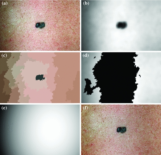
Methodology to estimate illumination map: a original image of a skin lesion, where the top edge is noticeably darker than the bottom edge; b illumination map determined via non-parametric modeling using Monte Carlo sampling; c segmentation map found using Statistical Region Merging; d regions included in the subset of skin pixels, where pixels black in colour are not classified as normal skin; e new illumination map determined by using (d) as a prior to the quadratic surface model; f resulting corrected image using the multi-stage illumination correction algorithm

Final Parametric Illumination Modeling

The initial non-parametric illumination model results in an estimate of the illumination variation in healthy skin, but does not properly model illumination near the lesion. Instead, the initial model identifies the lesion as a shadow. Using the initial model to correct the image would result in a significant bright spot around the lesion, which is obviously undesirable. To better model the illumination, a second stage is added, which results in a parametric model of illumination that uses the initial illumination pixel values. The parametric model can adequately estimate the illumination variation because illumination is assumed to change slowly throughout the image. The subset of pixels that are used to fit the parametric surface correspond to healthy skin in the original image.

To find the subset of healthy skin pixels, the original image is segmented into many regions. The segmentation algorithm used in this implementation is Statistical Region Merging [43]. The resulting segmented image is shown in Fig. 3c, where each region is represented as a single colour. Any regions that touched $20 \times 20$ pixel regions in the four corners of the image are considered part of the “healthy skin” class. While this method does not yield a perfect segmentation of the healthy skin and lesion classes, only an estimate of healthy skin pixels is required for fitting the parametric model. The regions that are considered ‘healthy skin” are shown in Fig. 3d.

The final illumination model $\hat{i}'$ is estimated as a parametric surface (4) with coefficients $$c_1$$

, which is fit to the initial illumination values $\hat{i}$ corresponding to pixels in the “healthy skin” subset $$S$$

using maximum likelihood estimation (5). The final parametric illumination model is shown in Fig. 3e.

$\begin{aligned} i'(x,y) = c_1 x^2 + c_2 x y + c_3 y^2 + c_4 x + c_5 y + c_6 \end{aligned}$

(4)

$\begin{aligned}&\hat{i}' = \mathop {\mathrm{argmax}}\limits _{\hat{i'}} \prod _{(x,y)\in S} P(\hat{i}(x,y) | \hat{i}'(x,y) )\\&\mathrm{where } P(\hat{i}(x,y) | \hat{i}'(x,y) ) \,\text {i.i.d.}\,\fancyscript{N}(\hat{i}'(x,y) , \sigma ^2) \nonumber \end{aligned}$

(5)

Reflectance Map Estimation

The reflectance map is calculated by dividing the V channel $$v$$

from the original image in the HSV colour space by $\hat{i}'$ . The reflectance map $\hat{r}$ replaces the original V channel and is combined with the original hue (H) and saturation (S) channels. The resulting image is corrected for illumination. An example of a corrected image is shown in Fig. 3f.

Feature Extraction

Once the image has been preprocessed, descriptive features are extracted to describe the lesion as a vector of real numbers. One of the most prominent clinical methods for diagnosing a skin lesion is using the ABCD rubric [41, 50], where the dermatologist looks for signs of asymmetry, border irregularity, colour variations, and diameter. However, this is done in a very subjective manner, and results in discrete categorical values. For example, the score assigned to a lesion’s asymmetry is determined by identifying whether the lesion is asymmetric across two orthogonal axes chosen by the dermatologist, resulting in a score $A \in \{0,1,2\}$ [50]. This type of subjective visual analysis leads to large inter-observer bias as well as some intra-observer bias [5]. We aim to create continuous high-level intuitive features (HLIFs) that represent objective calculations modeled on a human’s interpretation of the characteristic.

High-Level Intuitive Features

A “High-Level Intuitive Feature” (HLIF) is defined as a feature calculation that has been designed to model a human-observable phenomenon (e.g., amount of asymmetry about a shape), and whose score can be qualitatively intuited. As discussed in “Background”, most skin lesion features are low-level features. That is, they are recycled mathematical calculations that were not designed for the specific purpose of analysing a characteristic of the lesion shape.

Although designing HLIFs is more time-consuming than amalgamating a set of low-level features, we show in “Results” that the discriminative ability of a small set of HLIFs is comparable to a large set of low-level features. Since the HLIF set is small, the amount of required computation for classification decreases, and the risk of overfitting a classifier in a highly dimensional space is reduced, especially with small data sets.

In the next two sections, we describe nine HLIFs to evaluate the asymmetry and border irregularity of a segmented skin lesion. These HLIFs are designed to model characteristics that dermatologists identify. This work is described in detail in [3, 4], so we limit our analysis here to a general overview of the features.

Asymmetry Features

Dermatologists try to identify asymmetry with respect to shape or colour to indicate malignancy. These visual cues result due to the unconstrained metastasis of melanocytes in the skin.

HLIF for Colour Asymmetry

Asymmetry with respect to colour can be quantified by separating the lesion along an axis passing through the centre of mass (centroid) such that it represents the maximal amount of colour asymmetry. This “maximal” axis was found iteratively. First, we calculate the major axis of the lesion. The major axis is that which passes through the centroid and describes the maximal variance of the shape. The lesion image was then converted to the Hue-Saturation-Value (HSV) space so we can use the illumination-invariant hue measure to analyse the colours. The normalized hue histograms of both sides of the axis were smoothed using a Gaussian filter for robustness and were then compared to generate the following HLIF value:

$\begin{aligned} f_1^A = \max _\theta \left\{ \frac{1}{2} \sum _{i=1}^{nbins} |H_1^\theta (i) - H_2^\theta (i)| \right\} \end{aligned}$

(6)

where $H_1^\theta$ and $H_2^\theta$ are the normalized smoothed hue histograms according to the separation axis defined by rotating the major axis by $\theta$ , and $$nbins$$

is the number of discretized histogram bins used for binning hue values (we used $$256$$

bins). Noticing that $f_1^A \in [0,1]$ , $$f_1^A$$

can be intuited as an asymmetry score ranging from 0 (completely symmetric) to 1 (completely asymmetric).

Figure 4 depicts an example of this calculation. The lesion has a dark blotch on one side of it, rendering it asymmetric with respect to colour, which is reflected in the calculated value of $$f_1^A=0.3866$$

Fig. 4

Example of the design of $$f_1^A$$

by comparing the normalized hue histograms of both sides of the separation axis. The red bars represent the original binned histogram of hue values, and the blue line represents these histograms smoothed by a Gaussian function ( $\sigma =2$ bins), which allows us to compare hue histograms robustly. In this example, $$f_1^A=0.3866$$

, representing a lesion with asymmetric colour distributions. a Image separated by the axis that produces maximal hue difference. b Normalized hue histogram of the left side of the lesion. Note the prominence of blue pixels along with the red ones in the histogram due do the dark blotch in the image. c Normalized hue histogram of the right side of the lesion. Note the prominence of red pixels in the histogram in correspondence with the image. d Absolute difference of the two hue histograms. The amount of blue and lack of red pixels in the first histogram are reflected by the two “humps” in the difference histogram

HLIF for Structural Asymmetry

Making the observation that symmetry can usually not be found in highly irregular shapes, we express the segmented lesion as a structure and analyse its simplicity. Fourier descriptors apply the Fourier series decomposition theory to decomposing some arbitrary shape into low-frequency and high-frequency components. In particular, the points on the shape border are mapped to 1D complex number via $F:(x,y) \mapsto x + iy$ , where $$i$$

is the complex number. The Fourier transform is performed on this set of complex numbers. We can then compare a low-frequency (“simple”) reconstruction with the original shape to determine the amount of asymmetry due to shape irregularity.

First, since we must use the discretized Fourier transform, the lesion border was uniformly sampled at a fixed rate to ensure the same decomposition in the frequency domain across all images. The Fast Fourier Transform (FFT) was then applied, and only the two lowest frequency components were preserved. These two frequencies represent the zero-frequency mean and the minimum amount of information needed to reconstruct a representative border. The inverse FFT was applied on these two frequencies to reconstruct a low-frequency representation of the lesion structure. Comparing this shape with the original is ill-advised, as this would yield a metric that is more suitable for border irregularity. Instead, we applied the same procedure to reconstruct a structure using $$k$$

frequencies, were $$k$$

is some small number that reconstructs the general shape of the lesion. This shape is compared to the original shape to generate the following HLIF calculation:

$\begin{aligned} f_2^A = \frac{area(S_k \oplus S_2)}{area(S_k \bigcup S_2)} \end{aligned}$

(7)

where

and

are the

-frequency and $$2$$

-frequency reconstructions of the original lesion shape. This feature value can be intuited as a score representing the general structural variations. We found empirically that linearly sampling the border with $$1000$$

points and setting $$k=5$$

yielded good results.

Figure 5 depicts an example of this calculation. Notice how the lesion has a very abnormal shape that does not seem to contain any symmetry. The logical XOR (Fig. 5b) captures this structural variation, and the calculation represents the dark area with respect to the union in Fig. 5c.

Fig. 5

Example of the design of $$f_2^A$$

by comparing a baseline reconstruction of the lesion (magenta) with a low-frequency reconstruction (green) that incorporates the structural variability, it any exists. In this example, $$f_2^A=0.1609$$

, representing a structurally asymmetric lesion. a Original lesion, and reconstruction using 2 (pink) and 5 (green) frequency components. b Logical XOR of the two reconstructions (dark area). c Union of the two reconstructions (dark area)

Only gold members can continue reading. Log In or Register to continue