Information in Melanocytic Skin Lesion Analysis Based on Standard Camera Images

is defined over an $n \times m$ image , parameterized by an offset ( $\Delta x$ , $\Delta y$ ), as:

$\begin{aligned} \displaystyle C_{\Delta x, \Delta y}(i,j) = \sum _{p=1}^n \sum _{q=1}^m \left\{ \begin{array}{ll} 1, &{} if \;\; I(p,q) = i \;\; and \;\; I(p+\Delta x, q+\Delta y) = j \\ 0, &{} otherwise \end{array} \right. \!\!. \end{aligned}$

(1)

The indexes

and

, and consequently the size of

, are defined by the range of possible values in

. For instance, if

is binary, the generated co-occurrence matrix

has size of $2 \times 2$ , while a 24-bit color image generate a $2^{24} \times 2^{24}$ co-occurrence matrix. Usually, texture analysis methods compute these matrices for 8-bit grayscale images, frequently quantized for even less than 256 values, and are referred as gray-level co-occurrence matrices (GLCM).

Moreover, it should be observed that the ( $\Delta x$ , $\Delta y$ ) parametrization makes the co-occurrence matrix sensitive to rotation. Unless the image is rotated in 180 degrees, any image rotation will result in a different co-occurrence distribution. So, to achieve a degree of rotation invariance, usually texture analysis procedures compute co-occurrence matrices considering rotations of 0, 45, 90, and 135 degrees. For instance, if we are considering one single pixel offsets (a reference pixel and its immediate neighbour), four co-occurrence matrices are computed using $(\Delta x$ , $\Delta y) = \left\{ (1,0),\;(1,-1),\;(0,-1),\;(-1,-1)\right\}$ . This process is exemplified in Fig. 1 using an example image with four possible pixel values.

Fig. 1

Co-occurrence matrices computation example. a Reference example image; b–e Co-occurrence matrices for the rotations of $0^{\circ }$ , $45^{\circ }$ , $90^{\circ }$ and $135^{\circ }$ , respectively

Because co-occurrence matrices are typically large and sparse, these matrices are not directly used for image analysis. In 1973, Haralick et al. [19] proposed a set of 14 metrics (frequently referred as the Haralick features) computed through the co-occurrence matrices to represent the image textural patterns, and this set of metrics and other similar metrics proposed in the literature [12, 38] have been used in the last decades for many different applications.

As mentioned in section “Introduction”, textural features based on the co-occurrence matrices are also very frequently used in melanocytic lesions analysis, though not existing a default scheme for that. Celebi et al. [10], for instance, suggest to uniformly quantize the images to 64 gray levels, and then extract 8 Haralick features for each one of the four orientations using single pixel offsets. Iyatomi et al. [22] proposed using only 4 features, but 11 different offsets. While Celebi et al. and Iyatomi et al. applied these techniques on dermoscopy images, Alcón et al. [1] used the Haralick features for the quantification of the textural structures on standard camera images. However, Alcón et al. is probably the simplest algorithm, computing only 4 Haralick features using single pixel offsets. In our experiments (see section “Experimental Comparison of Texture Features for Melanocytic Skin Lesion Image Analysis”) we will follow the Celebi et al. algorithm, as described next, which in our opinion is the most complete procedure.

Celebi et al. [10] initially divide the image in three regions. Based on a predefined segmentation, it is defined the lesion region, an outer periphery and an inner periphery. These peripheral regions are defined as adjacent regions with areas equal to 20 % of the lesion area, respectively outside and inside the lesion region. To reduce the effects of segmentation inaccuracies, these peripheral regions omit areas equal to 10 % of the lesion area next to the lesion border. Then, the images are uniformly quantized to 64 gray levels, and co-occurrence matrices

considering the four orientations are defined for each one of three regions. Finally, these matrices are normalized (i.e., divided by the total of co-occurrences), and eight Haralick features [12, 19, 38] are computed:

$\begin{aligned} \displaystyle Maximum\;probability&= \max _{i,j} \; c(i,j) \;, \end{aligned}$

(2)

$\begin{aligned} Energy&= \sum _i \sum _j c(i,j)^2 \;, \end{aligned}$

(3)

$\begin{aligned} Entropy&= - \sum _i \sum _j p(i,j) \log (c(i,j)) \;, \end{aligned}$

(4)

$\begin{aligned} Dissimilarity&= \left| i-j \right| c(i,j) \;, \end{aligned}$

(5)

$\begin{aligned} Contrast&= \sum _{n=0}^{N-1} \left\{ \sum _i \sum _j c(i,j) \Bigg \vert \left| i-j \right| = n \right\} \;, \end{aligned}$

(6)

$\begin{aligned} Inverse\;difference&= \sum \frac{c(i,j)}{1 + \left| i-j \right| } \;, \end{aligned}$

(7)

$\begin{aligned} Inverse\;difference\;moment&= \sum \frac{c(i,j)}{1 + (i-j)^2} \;, \end{aligned}$

(8)

$\begin{aligned} Correlation&= \frac{(ij)p(i,j) - \mu _x \mu _y}{\sigma _x \sigma _y} \;, \end{aligned}$

(9)

where

is the value of the normalized co-occurrence matrix at indexes

is the number of gray levels, $\mu _x$ and $\mu _y$ are, respectively, the mean values of the rows and columns of

, $\sigma _x$ and $\sigma _y$ are the respective standard deviations, and in Eq. 6 the symbol $'\vert '$ indicates a condition that must be valid.

To obtain rotation invariant features, the 8 statistics are averaged over the four orientations, obtaining 24 features to represent the textural information in the three image regions. Celebi et al. also add the ratios and differences of the 8 statistics in each one of these regions, amounting 72 generated features for each single image.

In Celebi et al. experiments [10], these texture features were combined with 11 features based on the lesion shape and 354 color features to classify dermoscopy images. In section “Experimental Comparison of Texture Features for Melanocytic Skin Lesion Image Analysis” we present some experiments and discuss its performance to classify standard camera images using these texture features standalone.

Model and Pattern Oriented Methods

The objective of model and pattern oriented texture analysis methods is to capture the essence of the texture, not only describing this information but also synthesizing it [40]. We present next typical approaches based on those assumptions often used in melanocytic skin lesion analysis.

Fractal Features

Given a melanocytic skin lesion image, Manousaki et al. [26, 27] proposed to create a three-dimensional pseudo-elevation surface by using the image intensities. Attributing the value of 255 to black and 0 to white (i.e., the complement of the grayscale intensities) to the $$z$$

-coordinate component, the two-dimensional image ( $$I(x,y)$$

) is converted to 3D ( $$I(x,y,z)$$

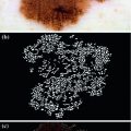
). Consequently, these pseudoelevations reveals delicate differences of texture within the lesions, and appear as spatial isotropic surfaces [27]. An example of the generated 3D fractal surface can be seen in Fig. 2.

Fig. 2

Pseudoelevation surface example. a Melanocytic skin lesion image; b 3D fractal surface generated from the lesion image

As we know, points, curves, surfaces and cubes are described in Euclidean geometry using integer dimensions of 0, 1, 2, and 3, respectively. A measure of an object such as the length of a line, the area of a surface and the volume of a cube are associated with each dimensions, and these measurements are invariant with respect to the used unit. However, almost any object found in nature appear disordered and irregular for which the measures of length, area and volume are scale-dependent. This suggests that the dimensions of such objects cannot be integers, i.e. these objects should be represented using fractal dimensions. For instance, a melanocytic lesion must have a dimension between 2 and 3, i.e. the dimension of an object that is not actually regular in shape and not a cube.

Many methods were proposed to compute the fractal dimension of an object [36]. The most used technique is probably the Minkowski–Bouligand dimension, also known as Minkowski dimension or box-counting dimension. Suposing the fractal on an evenly-space grid, we must count the number of boxes required to cover the object. The box-counting dimension is calculated by seeing how this number changes as we make the grid finer. Assuming $N(\varepsilon )$ as the number of boxes of side $\varepsilon$ required to cover the object, the fractal dimension $$D$$

is defined as:

$\begin{aligned} \displaystyle D = \lim _{\varepsilon \rightarrow 0} \; \frac{\log \, N(\varepsilon )}{\log \, (1/\varepsilon ) } . \end{aligned}$

(10)

In [27], Manousaki et al. used a modified algorithm of the Minkowski-Bouligand dimension proposed by Dubuc et al [16], using disks instead of boxes in its implementation. They performed experiments with 132 melanocytic skin lesion images, 23 of them being melanomas, 44 atypical nevi and 65 common nevi. While the melanomas achieved fractal dimension of 2.49 $\pm$ 0.10 (average $\pm$ standard deviation), the atypical nevi resulted 2.44 $\pm$ 0.11, and the common nevi resulted 2.46 $\pm$ 0.07.

In combination with fractal dimension, Manousaki et al. [26, 27] proposed the use of lacunarity parameter to classify the different textures. Lacunarity is a quantitative measure to describe differences in appearance of fractal surfaces with the same fractal dimension [25], measuring the distribution and size of “holes” within a textured surface.

Again, many different methods were proposed to compute the surface lacunarity [2]. Manousaki et al. suggested the gliding box method proposed by Allain and Cloitre [2]. A gliding box with size $r \times r$ is placed directly over the image and moves as a simple window, and the box mass $$M$$

is determined as the sum of the box content. The lacunarity at scale $$r$$

is defined as the variation of the computed $$M$$

values over the image divided by its square mean. Using the same image database with 132 lesion images, Manousaki et al. computed for melanomas lacunarity of 0.42 $\pm$ 0.35 (average $\pm$ standard deviation), while aytpical nevi resulted 0.25 $\pm$ 0.22, and common nevi resulted 0.19 $\pm$ 0.14.

Manousaki et al. did not experimented these computed textural descriptors in a classification step. However, they observed through statistical tests (Kruskal-Wallis and Mann-Whitney tests) that lacunarity can be potentially used to differentiate malignant and benign skin lesions, while fractal dimension do not provided significant statistical differentiation.

LBP Features

Local binnary pattern (LBP) is a texture operator that was proposed by Ojala et al. [30]. and has already been used for many different applications. This technique labels the pixels of an image by thresholding the neighborhood of each pixel based on its value, and generates a binary number to quantify the local texture. Let us consider the following $3 \times 3$ image to illustrate its functionality:

As can be observed in Fig. 3, all neighbor pixels with value higher or equal to the center pixel value assume ‘1’ in the LBP, while the neighbor pixels with lower value assume ‘0’. Arranging these 8 binary values in sequence we obtain a 8-digit binary number, i.e. the local texture of the $3 \times 3$ neighborhood can be represented by $$2^8 = 256$$

different labels. After computing the LBP for each image position, usually a histogram is used to describe the texture information of the whole image. This methodology also has been extended for larger neighborhoods, considering circles of larger radius and a large number of pixels [31].

Fig. 3

Local Binnary Pattern (LBP) computation example. a Reference example image; b Computed LBP (the 8 neighbor pixels are thresholded by the center pixel value)

However, if we observe again Fig. 3, it is obvious that the binary number generated from the neighborhood is dependent of the initial position to arrange the values. Although usually the clockwise direction is adopted, we can obtain 8 different numbers (or more, if larger neighborhoods are used). For instance, if we start at the top-left pixel we obtain $$00110100$$

, while we obtain $$01000011$$

if we start arranging from the bottom-right pixel. So, to create a rotation invariant descriptor, Ojala et al. proposed to generated all the possible binary numbers, and the resultant LBP is the minimum possible value. In this case, the minimum possible binary value is $$00001101$$

(i.e., starting the arrangement from the bottom-left pixel), and that would be the resultant rotation variant LBP to the example image in Fig. 3a.

Also, Ojala et al. proposed a step to reduce the feature vector. For instance, the 256 bins histogram can be a too high dimensional vector to be used in a posterior classification step. Considering that many applications use 16 neighbor pixels, the generated $2^{16} = 65,536$ bins histograms make unpractical the use of LBPs. So, they also proposed the concept of uniform pattern, which was inspired by the fact that some binary patterns occur more commonly in texture images than others. A LBP is called uniform if its binary number contains at most two bitwise transitions from 0 to 1 or vice versa. For example, the patterns $$00000000$$

(0 transitions), $$01110000$$

(2 transitions) and $$11001111$$

(2 transitions) are uniform whereas the patterns $$11001001$$

(4 transitions) and $$01010010$$

(6 transitions) are not. Since LBPs with lower number of transitions are much more frequent, the final histogram is computed in such way that all the non-uniform patterns are counted in a single bin. For instance, in the 256 possible patterns of a $3 \times 3$ neighborhood, 58 of which are uniform, and consequently the generated feature vector will be 59-dimensional. Moreover, if we consider the rotation invariant descriptors, this dimensionality is reduced to only 10 bins.

Zortea et al. [43] proposed to use LBPs for the texture analysis of melanocytic skin lesions. Although their experiments have been performed with dermoscopy images, we present their proposed algorithm here understanding that it is a valuable contribution to the literature. Moreover, our experiments (see section “Experimental Comparison of Texture Features for Melanocytic Skin Lesion Image Analysis”) indicate that this technique is a potentially useful also for standard camera images. Their algorithm starts by dividing the whole image in windows of $w \times w$ pixels, with 50 % overlapping of adjacent windows. Then, uniform rotation invariant LBPs of 16 neighbor pixels are computed, and a 18-dimensional feature vector is generated to each one of these windows. Finally, the whole set of computed features vectors is clustered in $$K$$

sub-classes (using the $$K$$

-means algorithm) and we obtain a dictionary of possible LBPs presented in melanocytic lesion images.

We may observe that there is no segmentation before the texture feature extraction, so the “skin” texture pattern is also presented in the generated dictionary of $$K$$

patterns. Zortea et al. understand that the “skin” pattern will be present in both malignant and benign classes, and consequently will not influence the posterior classification. Furthermore, that would make this technique not-dependent of segmentation inaccuracies.

So, after obtained the $$K$$

-dimensional texture dictionary, LBPs are computed in the testing image set, and the frequency of occurrence of each of the $$K$$

textural patterns is used as a textural representative vector. Additionally, they included a feature accounting the number of different patterns in each single image, providing a $$K+1$$

feature vector. The algorithm is based on the idea that malignant cases would generated higher frequencies for some textural patterns, while benign cases higher frequencies for different patterns of the dictionary.

In their experiments, Zortea et al. [43] used a Support vector machine (SVM) classifier with Radial Basis Function kernel and tested different parameters specification. The best classification results have been obtained using $$w=40$$

pixels and $$K=22$$

clusters, achieving sensitivity of 73.3 % and specificity of 73.9 %. In our experiments (see section “Experimental Comparison of Texture Features for Melanocytic Skin Lesion Image Analysis”), we randomly selected 30 images from each class for the computation of the texture dictionary, and we also varied the $$K$$

parameter to check the performance of these LBP features in a classification procedure.

Signal Oriented Methods

Many texture analysis techniques have been proposed relying on signal processing techniques, such as features computed from filtered images [40]. We present next two approaches often used for the melanocytic skin lesions analysis focused on that idea.

ICA Features

Tabatabaie et al. [39] proposed a filtering method based on independent component analysis (ICA) to describe the texture information of melanocytic skin lesion images. ICA is a method to construct independent components from an ensemble of data [34]. Let $$X$$