Fig. 1
General melanoma diagnosis process
Though data is the inalienable part of a computer aided diagnosis (CAD) system, the decision-making is of utmost importance, especially with the abundance of numerous imaging devices on the market. Here for a CAD system, decision-making refers to carrying a diagnosis based on certain algorithms/classifiers. In other words, a CAD system mimics the clinical diagnosis process, which typically involves computing techniques such as feature extraction and classification.
Although CAD based melanoma diagnosis has been an active research area, its clinical application is still stagnating currently. Before bringing CAD based melanoma inspection into real clinical practices, it seems there are two critical challenges which deserve highlights here:
There are a few publications covering the decision gap [2, 9, 18], which are of varying performances in dealing with the decision-making gap. However, to our knowledge, the data gap is still neglected by and large in CAD based melanoma diagnosis. To avoid data gap in CAD systems, it is important to choose attributes with equivalent metrics if numerical operations are going to be carried out between these attributes. In addition, numerical operations for attributes of different metrics shall be avoided.
(1)
Data gap: The feature descriptors describing pigmented lesion properties may include both metric and non-metric values. Some attributes might involve physical meanings such as the diameter, some other features, such as Euler number of the lesion area, might not have any unit. If this is the case, the decision-making process has data gap. Typical learning paradigms like support vector machines [11] and neural networks [9] treat these data as purely numerical ‘inputs’ without paying attention to the physical/clinical meanings of these attributes.
(2)
Decision-making gap: This refers to the decision making styles discriminating clinical diagnosis and computer based early diagnosis of melanoma. For instance, [1, 14, 21] only used border attributes in melanoma diagnosis. This decision-making style focuses on just one property of pigmented lesions. Though the one-feature based CAD is effective in justifying the usefulness of certain descriptors, there is a gap between these CAD systems and the clinical diagnosis.
In the literature, there are a few protocols proposed for decision-making in melanoma diagnosis.
In [9], a neural network was proposed to carry diagnosis of melanoma. The feature descriptors cover asymmetry/border/colour properties and overall there are 14 entries in the feature vector. In experiments, one of the tested neural networks includes 14 input neurons, 7 hidden neurons and 1 output neuron. This neural network was trained with the well-known back-propagation method.
Sboner et al. [17] formulated a multiple classifier system, including linear discriminant analysis (LDA), decision trees and k-nearest neighbor. The feature descriptors cover geometrical and colorimetric domains, resembling the ABCD rules proposed in [10].
In [18], another ABCD rules based system for melanoma diagnosis was tested. In this system, there are 8 feature descriptors: skin line direction, skin line intensity, asymmetry, border irregularity, red component variegation, green component variegation, blue component variegation and diameter of lesion. After dimension reduction for the feature vectors, the first two principal components of these 8 components are selected for designing a linear classifier. The area under the receiver operating characteristic (ROC) curve obtained is 0.94.
She et al. [18] represents a typical approach in designing computer aided diagnosis of melanoma, which involves dimension reduction after feature extraction. In [18] and [9, 17], there is one hidden assumption behind this method: different features representing different properties are numerically computable. Here by computable, it means they are allowed to be mixed together numerically, including addition/deduction etc. Due to the non-homogeneity of the attributes, this operation, though commonly accepted, neglects the data gap between different attributes. The associated undesirable risks include: Firstly, the result depends on the chosen metrics. Secondly, the result only has numerical meaning but the physical/clinical meaning might be elusive. For instance, suppose the skin line direction, blue component variegation and diameter of lesion are f , f
, f and f
and f respectively, adding them together as f
 +f
+f +f
+f gives a numerical number, which is hardly of any clinical significance.
, f and f respectively, adding them together as f+f+f gives a numerical number, which is hardly of any clinical significance.This chapter utilizes multiple decision trees for melanoma diagnosis, aiming at solving the data gap and the decision gap simultaneously. Section “Method” discusses the main designs of two multiple decision tree systems. Section “Experiments and Results” presents experimental results on a test dataset. For an early version of this paper, see [20].
Method
Since a typical decision-making process involves feature extraction and classification, this section is divided into two subsections. In section “Feature descriptors”, the shape, size and colour features for the pigmented lesions are examined, which are inspired by the ABCD rules [10, 16]. In section “Decision Trees”, unlike [17] which used three heterogeneous classifiers the decision tree is the only classifier employed here to conduct diagnosis.
Table 1
2D features for lesion images
Asymmetry | x1 |  | Asymmetry w.r.t. horizontal axis |
|---|---|---|---|
x2 |  | Asymmetry w.r.t. diagonal axis | |
x3 |  | Asymmetry w.r.t. off-diagonal axis | |
x4 |  | Asymmetry w.r.t. vertical axis | |
Border | x5 |  | Indentation irregularity index |
x6 |  | Protrusion irregularity index | |
x7 |  | Maximum indentation irregularity index | |
x8 |  | Maximum protrusion irregularity index | |
Colour | x9 |  | Colour variation in red channel |
x10 |  | Colour variation in green channel | |
x11 |  | Colour variation in blue channel | |
x12 |  | Colour variation in gray intensity | |
Diameter | x13 |  | Equivalent diameter |
x14 |  | Equivalent diameter of convex hull | |
x15 |  | First singular value of covariance matrix of coordinate vector | |
x16 |  | Second singular value of covariance matrix of coordinate vector |
Feature Descriptors
This is a classical topic in CAD based melanoma diagnosis. Here a set of features are extracted following the ABCD rules. As shown in Table 1, there are 16 attributes altogether.
Fig. 2
Extract asymmetrical features for suspicious pigmented lesions
Asymmetry
In [10], asymmetry rule means the more asymmetrical the lesion is, the more likely it is malignant. Celebi et al. and She et al. [7, 18] use principal axis based methods to describe the asymmetry features. In this chapter, a four-axis method is utilized to describe the asymmetry features. Figure 2 shows the idea of how to construct the asymmetry features. For instance, in Fig. 2a, the solid line is the first axis selected and the original lesion area lies within the region enclosed by the solid boundary. The dashed line encloses an area which, given the axis, is symmetrical with respect to (w.r.t.) the original lesion area. Apart from the horizontal line in Fig. 2a serving as the symmetrical axis, the diagonal line, off-diagonal line and vertical line can also be used as symmetrical axes. Figure 2b–d show these symmetrical axes and their corresponding symmetrical images of the original lesion area respectively.
To construct one symmetrical area as shown in Fig. 2, there are two steps. Firstly, one detects the centroid of the lesion area. Then a reference axis, i.e., the symmetrical axis, is selected. In Fig. 2, these symmetrical axes are 0, 45, 90, 135 degrees w.r.t. the horizontal axis. Denote the original lesion area as  , and the symmetrical lesion area as
  , the asymmetry indices are defined as:
where XOR means exclusive-or operation at pixel level; ‘#’ is to take the number of all non-zero elements. Thus these four attributes are all non-metric variables.
, and the symmetrical lesion area as , the asymmetry indices are defined as:(1)
Border Irregularity
To maintain the equivalence in terms of units for the border irregularity descriptors, indentation/protrusion index proposed in [14] is used here.
The method in [14] constructs an area based irregularity index in several steps: Firstly, a smoothed outline of the lesion is extracted via a series of multiscale Gaussian filters. Then the area enclosed within the smoothed outline is compared with the original lesion area. Denote the original lesion area as  and the smoothed area as
  , the indentation area lies within
  while outside
  . The protrusion area is the opposite: it lies within
  while outside
  . So the indentation and protrusion maps can be obtained as follows:
where  and
and  represents the indentation and protrusion images respectively. Specifically, for pixels in
  and
and  , the definitions are as follows:
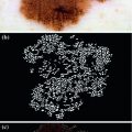 Network Detection and Analysis
 Analysis in Dermoscopic Images
 Skin Reflectance and Geometry for Diagnosis of Melanoma
 Diagnosis of Melanoma Based on the 7-Point Checklist
 Decision Support Using Lighting-Corrected Intuitive Feature Models
 Bag-of-Features Approach for the Classification of Melanomas in Dermoscopy Images: The Role of Color and Texture Descriptors


and the smoothed area as , the indentation area lies within while outside . The protrusion area is the opposite: it lies within while outside . So the indentation and protrusion maps can be obtained as follows:(2)
(3)
and represents the indentation and protrusion images respectively. Specifically, for pixels in and , the definitions are as follows:Related posts:
Network Detection and Analysis
Stay updated, free articles. Join our Telegram channel
Full access? Get Clinical Tree
