Basic Statistics

I. VARIABLES

A. Categorical variables (discrete variable)

1. Nominal variable: Variable with two or more categories but no intrinsic order. State of residence (Michigan, New York, etc.) is a nominal variable with 50 categories.

2. Dichotomous variable: A nominal variable with only two categories. Presence of diabetes (yes/no) and male/female are dichotomous variables.

3. Ordinal variable: Variables with two or more categories that can also be ordered or ranked. However, the orders or rank are not continuous variables (see below). Results from a Likert scale can be considered an ordinal variable (strongly agree/agree/neither agree or disagree/disagree/strongly disagree).

B. Continuous variables (quantitative variable)

1. Ratio variable: A variable that can be measured along a continuum and has a numerical value. A value of zero indicates that there is none of that variable. Examples include distance in centimeters or height in inches.

2. Interval variable: A variable that can be measured along a continuum and has a numerical value. A value of zero does not indicate absence of the variable. An example is temperature in degrees Fahrenheit, where a measurement of zero degrees does not indicate the absence of temperature.

C. For purposes of a study, there are two broad classes of variables

1. Independent variable (experimental variable or predictor variable): A variable that is observed or is being manipulated in an experiment or study

2. Dependent variable: The outcome of interest. A variable that is dependent or may be dependent on the independent variable(s).

II. WORDS TO KNOW

A. p Value: The likelihood that the observed association occurred due to chance alone. p < 0.05 is commonly considered “statistically significant.” When p = 0.05, what this is actually saying is that there is a 5% chance that the reported results occurred due to chance (or, that there is a 95% chance that the results are real)

B. α: The likelihood of a type I error

C. β: The chance of a type II error

D. Power: A study’s ability to detect a difference if one is present. A study’s power is calculated as 1-β

E. Null hypothesis: The null hypothesis typically refers to the default position, for example, that there is no association between two variables or that a treatment has no effect

1. The null hypothesis is often paired with an alternative hypothesis, which states that there is an association between two variables or that a treatment does have an effect

2. The null hypothesis can never be proven. The data to be analyzed will either reject or fail to reject the null hypothesis.

F. Type I error: The null hypothesis is rejected but the null hypothesis is actually true. The likelihood of a type I error is equal to your α value.

G. Type II error: Failure to reject the null hypothesis when the null hypothesis is false. The likelihood of a type II error is equal to your β value.

H. Standard deviation (SD) is a measure of the dispersion of values in a dataset from the mean. A low SD implies that values are clustered close to the mean. A high SD implies that values have wide dispersion around the mean.

1. Or, to put it another way, the SD reflects how close an individual observation will be to the sample mean

2. For a normal distribution, 68% of values lie within one SD and 95.5% within two SDs of the mean

I. Standard error of the mean (SEM) reflects how close the means of repeated samples will come to the true population mean for a given sample size. SEM is calculated by dividing the SD by the square root of sample size

J. Confidence interval: A range into which you are sure your data fall

1. Typically reported as a 95% confidence interval, for example, that you are 95% sure that the true value lies between the lower and upper borders of your interval

2. 95% confidence interval is calculated by taking the mean ± 1.96 × SEM

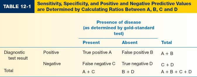
III. EVALUATING A DIAGNOSTIC TEST (Table 12-1)

A. Sensitivity measures a test’s ability to identify patients WITH disease

1. A test with high sensitivity is unlikely to give a false negative result

2. Sensitivity = A/(A + C)

B. Specificity measures a test’s ability to identify patients WITHOUT disease

1. A test with high specificity is unlikely to give a false positive result

2. Specificity = D/(B + D)

C. Positive predictive value (PPV) identifies the proportion of patients with a positive test result who actually HAVE the disorder. PPV helps determine how confident you are that your patient has the disorder. PPV = A/(A + B)

D. Negative predictive value (NPV) identifies the proportion of patients with a negative test result who do NOT have the disorder. NPV = D/(C + D)

IV. SAMPLE SIZE CALCULATION

A. This question is commonly asked: “How many patients do I need to determine if this intervention or treatment is effective?”

B. Prior to initiating the study, define the intervention and outcome of interest. Additionally, define your tolerance for type I and type II errors, typically 0.05 and 0.20, respectively.

1. For continuous outcome variables, you need an estimate of both mean and SD in the control and intervention groups

2. For dichotomous outcome variables, you need an estimate of event rate in the control and intervention groups

3. Pilot data (yours or someone else’s) are helpful to provide realistic estimates

C. Five values are required for sample size calculation for a dichotomous outcome. With these values, you (or your statistician) can calculate the number of patients required in groups 1 and 2.

1. α

2. Power

3. Expected event rate in group 1

4. Expected event rate in group 2

5. Ratio of patients in group 1 versus group 2 (typically 1:1)

D. Five values are required for sample size calculation for a continuous outcome. With these values, you (or your statistician) can calculate the number of patients required in groups 1 and 2.

1. α

2. Power

3. Expected mean and SD of outcome variable for group 1

4. Expected mean and SD of outcome variable for group 2

5. Ratio of patients in group 1 versus group 2 (typically 1:1)

V. STATISTICAL ANALYSIS

A. Univariate analysis looks for associations between two variables. Typically, one variable is a predictor variable and the second is an outcome variable.

1. t-test compares a variable’s mean value between two groups. Example: Mean BMI was significantly higher in patients who had a postoperative infection (30.9) when compared to patients who had no postoperative infection (24.8)

2. ANOVA can be used to compare a variable’s mean value between >2 groups. The Tukey t-test is used with an ANOVA to identify means that are significantly different from one another

3. Chi-squared test compares differences in proportions or observed rates between two groups. Example: The observed rate of DVT was significantly less in patients who received enoxaparin (4%) when compared to patients who did not receive enoxaparin (8%)

4. Fisher’s exact test is a variant of the chi-squared test that can be used when the total number of outcome events is low (<10)

B. Multivariable analysis examines the effect of an independent variable on an outcome of interest while controlling the effect of other variables

1. Logistic regression is performed dichotomous (yes/no) outcome variables. Example: When controlling for the effects of age, BMI, and smoking, presence of diabetes was an independent predictor of postoperative wound dehiscence

2. Linear regression is performed for continuous outcome variables (e.g., systolic blood pressure). Example: When controlling for the effect of diabetes, smoking, and activity level, increased age was an independent predictor of increased systolic blood pressure

C. Nonparametric statistics are required when the distribution of your outcome variable is not normal, or the variable itself is nonlinear

1. Example: Nonparametrics are required to examine Likert scale values, an ordinal variable. Likert scales are often arbitrarily assigned point values (e.g., strongly disagree (1), disagree (2), neither agree nor disagree (3), agree (4), and strongly agree (5)). However, these point values are not actually a continuous variable because they do not have units. Thus, you cannot use a t-test or linear regression techniques for analysis.

2. Examples of nonparametric statistics include the Wilcoxon rank–sum test, the Kruskal–Wallis one-way analysis of variance, and the Mann–Whitney U test

D. Parametric versus nonparametric statistics

1. Parametric statistics assume that the underlying distribution of the variables is normal

2. Nonparametric statistics make no assumption about distribution of the variables

VI. DESCRIPTION OF RESULTS

A. Incidence: The rate of an event in a distinct time period. Example: 230,000 new cases of breast cancer will be diagnosed in 2012

B. Prevalence: The number or proportion of individuals in a population who have a disorder at any time point. Example: 20% of individuals over the age of 65 have medication-controlled diabetes

C. Relative risk: The risk of an adverse event relevant to exposure. Calculated as (disease rate in exposed patients)/(disease rate in nonexposed patients).

D. Odds ratio: A description of strength of association between two variables, typically a predictor and outcome variable

1. Odds ratio is a measure of effect size and is commonly reported in logistic regression analysis. If the 95% CI for an odds ratio crosses 1, there is no significantly independent association.

2. Odds ratio is often confused with relative risk but the two are very different

E. Risk versus odds

1. For rare events (<10% incidence), risk and odds are essentially identical. For more common events, this is not true.

2. Example: Consider a deck of 52 playing cards. The risk of pulling an ace is 4/52. The odds of pulling an ace are 4/48. For rare events, OR and RR are very close. However, the risk of pulling a black card is 26/52. The odds of pulling a black card are 26/26. For common events, OR and RR are not similar.

F. Absolute risk reduction (ARR): (Event rate in control group) − (event rate in intervention group). This is the real measure of effect size

G. Relative risk reduction: ARR/(event rate in control group). Relative risk reduction can be misleading. For example, a drug that decreases an event rate from 0.1% to 0.075% has a 25% relative risk reduction but an absolute risk reduction of only 0.025%.

H. Number needed to treat: The number of patients that must be treated to prevent one adverse outcome. Calculated as the inverse of ARR. NNT = 1/ARR

I. Number needed to harm: The number of patients who need to receive a treatment to have one adverse event

1. Calculate the absolute adverse event rate: (adverse event rate in the intervention group) − (adverse event rate in the control group)

2. NNH = 1/(absolute adverse event rate)

VII. STATISTICAL SIGNIFICANCE VERSUS CLINICAL IMPORTANCE

A. Do not always focus on statistical significance. Remember, by definition, the p-value indicates the likelihood that the observed association was due to chance alone. The p-value says nothing about the importance or relevance of a relationship.

B. Statistical significance is a measure of confidence. Effect size is a measure of importance

C. Statistically significant differences can be clinically meaningless. Large database studies often show significant differences among clinically irrelevant results (like a BMI of 29.8 in the control group and BMI of 30.0 in the intervention group).

D. Nonstatistically significant differences can still have a large effect size. When differences are large but the differences were not significant, this represents an underpowered study (e.g., sample size was too small, also known as a type II error). These studies can be used as excellent pilot data for your own, larger study

PEARLS

1. Investigators who do not have a formal background in statistics should collaborate with a statistician in all phases of a research project

2. For dichotomous outcome variables, sample size calculation requires an estimate of the event rate in the control and treatment groups

3. For continuous outcome variables, sample size calculation requires an estimate of the mean and standard deviation for the outcome variables in the control and treatment groups

4. Pilot data are incredibly helpful in sample size calculation

5. Statistical significance is not the same as clinical relevance

QUESTIONS YOU WILL BE ASKED

1. Describe the difference between sensitivity and specificity.

Sensitivity examines a test’s ability to find patients WITH disease. Specificity examines a test’s ability to find patients WITHOUT disease.

2. What is a type 1 error and a type 2 error?

A type I error rejects the null hypothesis when the null hypothesis is actually true.
A type II error fails to reject the null hypothesis when the null hypothesis is false.

3. What is the difference between incidence and prevalence?

Incidence refers to a disease rate within a certain time period (e.g., rate of post-operative MI at 30 days). Prevalence refers to the proportion of the overall population who has disease at a certain time point. Incidence looks at NEW disease. Prevalence looks at ALL disease.