Bag-of-Features Approach for the Classification of Melanomas in Dermoscopy Images: The Role of Color and Texture Descriptors

93 % and Specificity 88 %. Furthermore it shows that color descriptors perform better than texture ones in the detection of melanomas.

Keywords

Melanoma diagnosisDermoscopyBag-of-features Feature extractionFeature analysisColor features Texture features

Introduction

Dermoscopy is a widely used microscopy technique for the in-vivo observation of skin lesions. A magnification instrument is used to increase the size of the lesion and a liquid (oil, alcohol or water) is placed on top of the lesion prior to the observation to eliminate surface reflection. This step makes the cornified layer of the skin translucent, allowing a better visualization of several pigmented structures located within the epidermis, dermis and dermoepidermal junction [3]. Several magnification instruments are currently used by dermatologists: dermatoscope, stereomicroscope or a digital acquisition system. The later allows the attainment of dermoscopy images, that can be processed and analyzed by a Computer Aided-Diagnosis (CAD) system.

The diagnosis of pigmented skin lesions using dermoscopy is based on medical algorithms: ABDC rule [47], 7-point checklist [2] and Menzies’ method [29]. All of these methods have in common a set of dermoscopic criteria that can be divided in two groups. The first group is called global features and allows a preliminary and quick categorization of a skin lesion. Global features are a set of patterns (reticular, cobblestone, globular, parallel, etc) that can be found in different pigmented skin lesions. The other group of dermoscopic criteria are the local features (pigment network, dots and globules, streaks, pigmentation related structures, vascular pattern, etc). These features are sometimes called the letters of the dermoscopic alphabet since they are the cues that allow a final diagnosis of the lesion (melanoma or not) [3]. Figure 1 illustrates some of the local dermoscopic features.

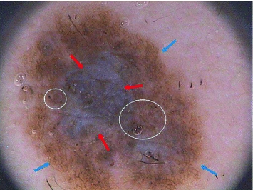
Fig. 1

Melanoma with specific dermoscopic features: blue-whitish veil (red arrows); pigment network (blue arrows), dots and globules (white circles)

Both global and local features play an important role in the diagnosis of melanomas. Some dermatologists perform an analysis of skin lesions using as reference only the global dermoscopic features. This global evaluation method is called pattern analysis and has received some attention in the skin research area, such as [1, 36, 40], which try to reproduce the medical analysis. The published works focus on the identification of the different patterns but do not perform a diagnosis of a skin lesion. However, it is undeniable that local features are the backbone of the common medical algorithms since ABCD rule, 7-point checklist and Menzies’ method use these features and their properties (shape or number of colors) to score a skin lesion, thus diagnosing it as melanoma or not. There are several studies which focus on detecting one or more of these dermoscopic criteria, such as pigment network [6, 37], irregular coloration [10, 31, 45], irregular streaks [35] and granularity [46]. However, as far as the authors know only one study combines a set of detectors and the 7-point checklist algorithm in a CAD system to perform a diagnosis using dermoscopy images [15]. Two reviews on state-of-the art methods can be found in [11, 25].

Most of the CAD systems found in literature use a different procedure, following a pattern recognition approach to classify dermoscopy images [9, 18, 21, 34]. These works have successfully exploited a global representation of the lesion using features inspired by the ABCD rule (color, shape, texture and symmetry). Most of the extracted features are able to perform a good description of the lesion regarding its shape and global color distribution. However, localized texture and color patterns associated to differential structures (e.g., pigment network, dots, streaks or blue-whitish veil) might be missed since a global analysis is being performed. To overcome this situation, this chapter describes a different approach for the analysis of dermoscopy images. Since experts usually try to characterize local structures in the image, the described strategy will try to mimic this behavior and represent the image by a set of local features, each of them associated to a small region in the image. The local features used describe the texture and color of each region and a comparative study between the two types of descriptive features is performed, in order to assess their degree of discrimination.

Bag-of-Features

The description of an image with local features have been successfully used in several complex image analysis problems, such as scene recognition and object-class classification [22, 23, 27, 42, 44, 50]. The used approach is called Bag-of-Features (BoF) [42, 44] and it is inspired by the bag-of-words (BoW) [5], which is a well known text retrieval algorithm. The procedure used by BoW to model documents evolves in three different steps. The first step consists of parsing the documents of the dataset into words, i.e., dividing the documents to smaller components. Images can also be sampled into smaller regions (patches). Two sampling strategies are commonly used in BoF: sparse and dense sampling. Sparse sampling is performed by detecting a set of informative keypoints (e.g., corners) and their respective support regions (square patches). This detection can be done using one or more of the several detectors proposed in literature (e.g. Difference of Gaussian [28] or Harris-Laplace [30]). A comparative study between the six most popular keypoint detectors can be found in [22]. For dense sampling it is assumed that each keypoint is the node of a regular grid defined in the image domain. The patches associated with the keypoints are extracted by sampling uniformly over the grid. Both sampling methods have been used in different works and a comparison between the two strategies was performed by van de Sande et al. [38]. Their experimental results showed that dense sampling outperformed sparse sampling. The BoF approach proposed in this work uses dense sampling to extract the patches from a given image and only patches whose area is more than 50 % inside the lesion are considered.

The second step in BoW document analysis is to represent each word by its stem. The equivalent for the image analysis case is to represent each patch by a feature vector $x_{i}\in \mathbb R ^n$ . Different features can be used to locally describe the patches. This chapter focus on two specific kinds of features, color and texture, which will be addressed in section “Local Features”. $$N$$

square patches are extracted from each image $$I$$

on the dataset. Therefore, a family of local features will be associated with $$I$$

as follows

$\begin{aligned} F = \left\{ x_1, \ldots , x_N \right\} ,\quad x_i\in \mathbb R ^n. \end{aligned}$

(1)

The last step of both BoW and BoF corresponds to the training process. In the first, each discriminative word receives an unique label. Very common words, which occur in most documents, are rejected and do not receive a label. This process can be seen as the creation of a dictionary of representative words. Then, each document is analyzed separately and its discriminative words are compared with the ones from the dictionary. From this comparison will result an histogram of the frequency of occurrence of the dictionary words within the document. This histogram will represent the document and will be used to compare different documents and assess their degree of similarity. Reproducing this histogram representation in the BoF case requires some extra effort. First, assuming that there is a dataset of $$L$$

images, this dataset has associated with it set of all the extracted local features

$\begin{aligned} {\fancyscript{F}} = \bigcup _{k=1}^L F^{(k)}. \end{aligned}$

(2)

In practice, the set ${\fancyscript{F}}$ has many thousands (or even millions) of feature vectors. Therefore, in order to obtain a visual dictionary (analogous to the dictionary of BoW), this set has to be approximated by a collection of prototypes $c_{1},\ldots ,c_{K},$ called visual words. The visual words are obtained using a clustering algorithm (in this work K-means is used). After obtaining a visual dictionary, all feature vectors in the training set are classified in the nearest visual word and a label

$\begin{aligned} l^{(k)}_i = \arg \min _j \Vert x^{(k)}_i - c_j\Vert , \end{aligned}$

(3)

which identifies a specific visual word, assigned to each feature vector $x^{(k)}_i$ . The final step is to characterize each image $I^{(k)}$ by a histogram of visual words frequency

$\begin{aligned} h^{(k)}(l) = \frac{1}{N^{(k)}}\sum _{i=1}^{N^{(k)}} \delta (l^{(k)}_i - l), \end{aligned}$

(4)

where $\delta (.)$ denotes the Kronecker delta ( $\delta (x)=1$ , if $$x=0$$

; $\delta (x)=0$ , otherwise). As in BoW, this histogram will act as the feature vector that describes the image and the set of $$L$$

feature vectors obtained this way will be used to train a classifier.

Fig. 2

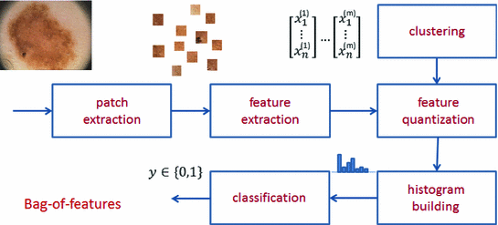
Block diagram of the BoF classification system

For each new image $$I$$

to be classified the process is similar to the one described previously. The image is sampled and local features are extracted. Then, the local features are compared with the dictionary of visual words obtained in the training phase and, finally, the histogram of visual words frequency is computed. The image is classified using the computed histogram and the classifier learned using the training set.

All the steps of the BoF strategy described previously are summarized in Fig. 2.

There are several factors that can impact the performance of BoF. Following the blocks sequence on Fig. 2 these factors are: the size of the regular grid ( $\delta$ ) used in the patch extraction step, the type and quantity of extracted features, the size of the dictionary ( $$K$$

), and the classification algorithm used. All these factors are thoroughly analyzed in this work. Several values for $\delta$ and $$K$$

are tried and three classification algorithms with different properties are tested: k-nearest neighbor (kNN) [16], AdaBoost [17] and support vector machines (SVM) [8, 12].

Local Features

The local dermoscopic criteria used by dermatologists to diagnose skin lesions can be represented by two different kinds of image features: texture and color features. Local dermoscopic structures such as pigment network, dots and streaks can be characterized by texture features since these features represent the spatial organization of intensity in an image, allowing the identification of different shapes. Color features describe the color distribution, thus they are able to characterize particular pigmented regions such as blue-whitish veil or regression areas.

In theory both of these features provide a good description of the extracted patches (see Fig. 2) and both play an important role in the final classification. One of the main objectives of this chapter is to determine if the previous hypothesis are correct. This objective is accomplished by assessing the performance of color and texture features separately and by combining both of them. Moreover, since both color and texture features can be extracted using different types of descriptors, a comparison between some of them is also performed. The several texture and color descriptors tested are described in the next sections.

Texture Descriptors

Texture features characterize the intensity of an image. Therefore, it is necessary to convert the original RGB image into a gray level one before extracting texture descriptors. This is done by selecting the color channel with the highest entropy [41].

Texture descriptors can be divided into several categories depending on the methodology used. This chapter focus on three different methods: statistical, signal processing and gradient [33]. In statistical methods, the features are extracted by computing neighbor pixel statistics. A very well known method for computing these statistics is the gray level co-occurrence matrix (GLCM) proposed by Haralick et al. [20]. This matrix stores the relative frequencies of gray level pairs of pixels at a certain relative displacement and can then be used to compute several statistics which will be the elements of the feature vector. The results presented in this chapter are obtained using five of the most common statistics: contrast, correlation, homogeneity, energy and entropy. The performance of these features is directly related with GLCM, since it has been already proved that the performance of a classification system is influenced by the number of gray levels ( $$G$$

) used as well as the way of combining the orientations of the nearest neighbors [13]. Therefore, several values of $$G$$

and two ways of combining the orientations (average GLCM versus four GLCM) are tested, according to what is proposed in [13].

Signal processing approaches have in common three sequential steps. First, the image $$I(x,y)$$

is convolved with a bank of $$N$$

filters, with a certain impulse response $h_{i}(x,y), \;\ i=1,\ldots ,N$ . Then, an energy measure of the output $J_{i}(x,y)\;\ i=1,\ldots ,N$ , is performed

$\begin{aligned} E_{i} = \sum _{x}\sum _{y}|J_{i}(x,y)| . \end{aligned}$

(5)

Finally, the energy content is used to computed statistics that are the components of the feature vector [33]. The two statistics computed in this chapter are the mean $\mu _{i}$ and standard deviation $\sigma _{i}$

$\begin{aligned} \mu _{i} = \frac{E_{i}}{M}, \quad \sigma _{i} = \sqrt{\frac{E_{i}-\mu _{i}}{M}}, \end{aligned}$

(6)

where

is the number of pixels $$(x,y)$$

in $J_{i}$ .

Several filter banks can be found on literature [33]. This chapter compares two of the most well known: Laws [26] and Gabor [4] filter masks. The filter masks proposed by Laws [26] have been widely used for texture characterization. These masks can have a dimension $3\times 3$ or $5\times 5$ and result from convolving two of of the five possible 1-D kernels. Each 1-D kernel focus on specific textural characteristics like edges, waves or ripples. In this chapter only three kernels will be used: $$L$$

, which computes the average grey Level, $$E$$

that extracts Edges (describe linear structures, such as pigment network) and $$S$$

that extracts Spots (describe circular structures, such as dots). The 1-D kernel values are the following: $L_{3} = [1\; 2\; 1], \; E_{3} = [1\; 0 \;-1], \; S_{3} = [1 \; -2 \; 1], \; L_{5} = [1 \;\ 4 \;\ 6 \;\ 4 \;\ 1],\; E_{5}=[-1 \;\ -2 \;\ 0 \;\ 2 \;\ 1]$ and $S_{5}=[-1\;\ 0 \;\ 2 \;\ 0 \;\ -1]$ . All the possible combinations of 1-D kernels are considered, thus the filter bank has a dimension $$N=9$$

. Since it is not known the dimension of the masks that leads to the best results, both $3\times 3$ and $5\times 5$ filter banks are tested.

Gabor filters have been used for texture classification [4] and edge detection [19]. Therefore, they can be used to characterize dermoscopic structures that have a linear shape (e.g. pigment network or streaks). The impulse response of a Gabor filter is the following

$\begin{aligned} h_{i}(x,y) = e^{\frac{\tilde{x}^{2}+\gamma ^{2}\tilde{y}^{2}}{2\sigma _{G}^{2}}}\cos \left( 2\pi \frac{\tilde{x}}{\lambda }+\varphi \right) , \end{aligned}$

(7)

where $\gamma$ is an aspect ratio constant. $\sigma _{G}$ is the standard deviation, $\lambda$ is the wavelength, $\varphi$ is the phase of the filter and $(\tilde{x},\tilde{y})$ are obtained from rotating $$(x,y)$$

as follows [19]

$\begin{aligned} \tilde{x} = x\cos \theta _{i}+y\sin \theta _{i},\qquad \tilde{y}=-x\sin \theta _{i}+y\cos \theta _{i}. \end{aligned}$

(8)

The angle amplitude $\theta _{i} \in [0,\pi ]$ determines the orientation of the filter $h_{i}$ and the step between two consecutive filters is $\frac{\pi }{N_{\theta }}$ , where $N_{\theta }$ is the number of filters in the filter bank [19]. This descriptor depends on several parameters. In this chapter two of them are varied: $\sigma _{G}\in \{1,2,\ldots ,5\}$ and $N_{\theta }\in \{2,3,\ldots ,10\}$ . All the others are kept constant and equal to: $\gamma =0.5$ , $\varphi =0 \; rad$ and $\frac{\tilde{x}}{\lambda }=0.56$ [19].

Fig. 3

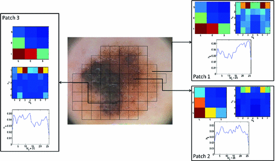
Texture features for three different $60\times 60$ patches: energy content for Laws ( $5\times 5$ masks) and Gabor ( $N_{\theta }=1,2,\ldots ,7$ and $\sigma _{G}=1,2,\ldots ,5$ ) filters and histogram of the gradient phase ( $M_{\phi }=25$ )

Gradient features such as gradient histograms have also been successfully used in several classification problems [14, 28]. In this work, two gradient histograms are used: amplitude and orientation. The image gradient $g(x,y)= [g_{1}(x,y) \;\ g_{2}(x,y)]$ is computed using Sobel masks. Then, gradient magnitude and orientation are respectively computed as follows

$\begin{aligned} \parallel g(x,y) \parallel = \sqrt{g_{1}(x,y)^{2}+g_{2}(x,y)^{2}}, \phi (x,y) = \tan ^{-1} \left( \frac{g_{2}(x,y)}{g_{1}(x,y)} \right) . \end{aligned}$

(9)

Finally, the histograms of gradient amplitude and orientation are obtained

$\begin{aligned} h_a(i)&= \frac{1}{N} \sum _{x}\sum _{y} b_i(\Vert g(x,y)\Vert ),\qquad i=1, \dots , B_a, \nonumber \\ h_{\phi }(i)&= \frac{1}{N} \sum _{x}\sum _{y} \tilde{b}_i(\phi (x,y)), \qquad i=1, \dots , B_\phi , \end{aligned}$

(10)

where

is the number of pixels inside the patch and $B_{a}, B_{\phi }$ are the number of bins of the magnitude and orientation histograms, respectively. Finally, $b_{i}(.), \tilde{b}_{i}(.)$ are the characteristic functions of the $$i$$

th histogram bin

$\begin{aligned} b_i(a)=\left\{ \begin{array}{ll}1 &{} \mathrm {if} a \text {belongs to the}i\text {th amplitude bin} \\ 0 &{} \text {otherwise}\end{array}\right. \nonumber \\ \tilde{b}_i(\phi )=\left\{ \begin{array}{ll}1 &{} \text {if} \phi \text {belongs to the} i\text {th orientation bin} \\ 0 &{} \text {otherwise}\end{array}\right. . \end{aligned}$

(11)

The parameter varied for both gradient features is the number of bins of the histograms ( $B_{a} \in \{15,25,35,45\}$ and $B_{\phi } \in \{15,25,35,45\}$ ).

Figure 3 shows some of the extracted texture features for three different patches within the same lesion. The exemplified patches were selected in order to include a specific dermoscopic structure: pigment network (patch 1), dots (patch 2) and globules (patch 3). It is clear that the extracted descriptors (Laws, Gabor and $h_{\phi }$ ) are different for each patches, which demonstrates that different dermoscopic structures have different textural properties and, therefore, must be described separately.

Color Descriptors

Several color descriptors, such as histograms and mean color, have been used in object and scene recognition problems [39]. The descriptors are usually computed over one or more color spaces like RGB, HSV/I [49], CIE La*b* and L*uv [49] and the biologically inspired opponent color space (Opp) [7]. These six color spaces have different properties, thus they might provide different information for the melanoma classification problem addressed in this chapter. For this reason the six previous color spaces are tested.

For each color space a set of three histograms is computed (one for each of the three color components). For each patch, the histogram associated with the color channel $I_{c}, \; c \in \{1,2,3\}$ is given by

$\begin{aligned} h_c(i) = \frac{1}{N} \sum _{x,y} b_c(I_{c}(x,y))\; i=1, \dots , B_c, \end{aligned}$

(12)

where

is the number of pixels inside the patch, $$i$$

is the histogram bin, $B_{c}$ is the number of bins and $b_{c}(.)$ is the characteristic function of the $$i$$

th bin

$\begin{aligned} b_c(I_{c}(x,y))=\left\{ \begin{array}{ll}1 &{} \mathrm {if} I_{c}(x,y) \text {belongs to the} i\text {th color bin} \\ 0 &{} \text {otherwise}\end{array}\right. . \end{aligned}$