Basic Mathematics in Skin Absorption

Symbol

Generic units

Description

m²

Area of application

AUC

kg/m³

Area under the curve

kg/m³

Concentration

c _ss

kg/m³

Steady-state concentration

C ₀

kg/m³

Initial concentration at

m³/h

Systemic clearance

m²/s

Diffusion coefficient

h _v

Height of applied formulation

$\frac{\mathrm{mol}}{m^2 s}$

Diffusion flux

J _max

$\frac{\mathrm{mol}}{m^2 s}$

Maximum diffusion flux

J _peak

$\frac{\mathrm{mol}}{m^2 s}$

Peak flux

J/K

Boltzmann’s constant

Partition coefficient

K _o/w

Octanol–water partition coefficient

k _p

m/s

Permeability coefficient

k _t

$\frac{\%\kern0.5em \mathrm{applied}}{s}$

Transfer coefficient

(Macroscopic) thickness

Mass

Mass per area

M _ss

Steady-state amount of solute in the membrane

${M}_{\infty }$

Applied mass

Molecular weight

ODE

Ordinary differential equation

Pharmacokinetic

Radius

Saturation concentration

Time

t _lag

Lag time

t _peak

Time to peak flux

Temperature

m³

Volume

Space

Pa s

Viscosity

$\frac{\mathrm{J}}{\mathrm{mol}\kern0.5em \mathrm{K}}$

Chemical potential

1.1 Mathematical Background of Analyzing Skin Absorption Processes

It is usually assumed that the travel of molecules through the skin membrane is governed simply by passive diffusion due to the absence of active transporters. From an atomistic point of view, diffusion is based on Brownian motion of particles in virtue of their thermal energy. From an empirical and more macroscopic understanding, the driving force of molecular movement is a concentration gradient of the diffusant in a medium and can be mathematically described by laws derived by Adolf Fick in 1855.

Fick’s first law (Eq. 1.1) relates the diffusion flux J (e.g., in mol/m² s) to the concentration gradient. Here, D, the diffusion coefficient, is a proportionality constant usually given in m²/s, and c the concentration at point x in space and time t.

$J\left( x, t\right)=- D\kern0.5em \nabla c\left( x, t\right)$

(1.1)

Assuming conservation of mass, one can derive Fick’s second law of diffusion (Eq. 1.2):

$\frac{\partial c\left( x, t\right)}{\partial t}=\nabla \left( D\kern0.5em \nabla c\left( x, t\right)\right)$

(1.2)

In this general equation, the diffusion coefficient may vary in dependence of location and/or concentration. Additional terms can be included to address, for example, binding phenomena (Frasch et al. 2011), enzymatic reactions (Guy et al. 1987), corneocyte desquamation (Reddy et al. 2000a, b), or general convective transport to model elimination or clearance of molecules into the systematic circulation (Dancik et al. 2012). For the one-dimensional case and a homogenous medium (constant diffusivity), (Eq. 1.2) simplifies to Eq. 1.3

$\frac{\delta c\left( x, t\right)}{\delta t}= D\frac{\delta^2 c\left( x, t\right)}{\delta {x}^2}$

(1.3)

Homogeneity is often a strong simplification but a typical assumption for easy analytical models to describe transdermal drug transport. Solutions of these parabolic partial differential equations can be solved analytically for various initial and boundary conditions and are presented in Sect. 1.3. As mentioned earlier, these conditions often denote simplifications and are only true for the description of a specific experimental setup (e.g., infinite dose or finite dose conditions with certain initial conditions). This is a fundamental issue and must be always kept in mind when applying mathematical models in general. We will shortly discuss more flexible but complex models in Sect. 1.5 that allow the application to a wider range of scenarios.

For the inhomogeneous and more general case, the diffusion flux at a cross section x at time t is directed from sites of higher chemical potential to sites of lower chemical potential ((Eq. 1.4 (Crank 1975); Anissimov and Roberts 2004)). Inhomogenous media transitions change the classical diffusion problem to a diffusion-partition problem.

$J\left( x, t\right)=-\frac{D}{kT} c\left( x, t\right)\frac{\delta \varphi \left( x, t\right)}{\delta x}$

(1.4)

Here, φ(x, t) is the chemical potential of the substance, T is the temperature, and k is Boltzman’s constant. For the homogeneous case with $\varphi \left( x, t\right)= kT \ln ( c\left( x, t\right)$ and a constant diffusivity, Eq. 1.4 simplifies to the standard diffusion equation as stated in Eq. 1.3.

The general case equation that describes the diffusion-partition problem with the chemical potential defined as $\varphi \left( x, t\right)= kT \ln \Big(\left( c\left( x, t\right)/ K(x)\right)$ _, and the position-dependent partition coefficient K is given by Eq. 1.5 (Anissimov and Roberts 2004):

$\frac{\delta c\left( x, t\right)}{\delta t}=\frac{\delta}{\delta x}\left(\begin{array}{l} D(x)\frac{\delta}{\delta x} c\left( x, t\right)\\ {}- D(x) c\left( x, t\right)\frac{\delta}{\delta x} \ln K(x)\end{array}\right)$

(1.5)

Besides studies with variable partition and/or diffusion coefficients inside a certain skin layer (Anissimov and Roberts 2004), it is more common (especially for more complex multilayer models) to assign specific diffusion coefficients to the different layers and specific partition coefficients to the interfaces of two adjacent layers. In this chapter, the presented solutions of the diffusion equation and determination of distinctive parameters almost exclusively depend on predicted, fitted, or experimentally determined diffusivities and partition coefficients. Therefore, at least a basic understanding of the relationship between molecular properties and the aforementioned parameters is essential when it comes to the preparation, setup, and evaluation of transdermal skin transport.

For spherical particles in a continuous fluid, the diffusion coefficient can be calculated by using the well-known Stokes–Einstein relation (Eq. 1.6), with viscosity of the solvent η and particle radius r:

$D=\frac{kT}{6\pi \eta r}$

(1.6)

For diffusion in polymers, it could be found empirically that for a small particle the following relationship holds (Eq. 1.7) (Anderson and Raykar 1989):

${D}_m={D}_m^0 M{W}^{- n}$

(1.7)

Here, MW is the solute molecular weight, and n and D _m⁰ are constants, the characteristics of the membrane at a specific temperature. Other theories derived from polymer research have also been applied successfully to the field of describing diffusivities in the skin domain. For deeper insight, the interested reader is kindly referred to Hansen et al. (2013).

Where the diffusivity D denotes the speed of a diffusant through a membrane and is inversely related to the weight of the solute, the partition coefficient K accounts for jumps in concentrations at the interface of two adjacent skin layers and is often related to a measure of solute lipophilicity, most commonly the logarithmic octanol–water partition coefficient. K is a thermodynamic parameter reflecting the relative affinity of a solute for a certain phase over another phase. Hence, the partition coefficient between layer m ₂ and layer m ₁ can be defined as Eq. 1.8

${K}_{m_2/{m}_1}=\frac{C_{m_2}^{\mathrm{eq}}}{C_{m_1}^{\mathrm{eq}}}$

(1.8)

with ${C}_{m_2}^{\mathrm{eq}}$ and ${C}_{m_1}^{\mathrm{eq}}$ being the respective solute concentrations at the interface of the two adjacent phases at equilibrium. In general, the partition coefficient is concentration-dependent, but if the solubilities in the two phases are relatively low (which holds true for many cases), this effect can be neglected, and the partition coefficient can be defined by using the saturation concentrations ${S}_{m_1}$ and ${S}_{m_2}$ in the different layers (Anissimov et al. 2013), with Eq. 1.9

${K}_{m_2/{m}_1}=\frac{S_{m_2}}{S_{m_1}}$

(1.9)

A typical strategy is to establish a relationship between an easy-to-observe parameter that mimics the membrane properties and the parameter of interest. A prominent example is the ocanol/water partition coefficient K _o/w that could be related to the stratum corneum lipid phase/water partition coefficient K _lip _,with the help of a linear free-energy relationship (Eq. 1.10) (Anderson et al. 1988)

${K}_{\mathrm{lip}}= a{K}_{o/ w}^b$

(1.10)

Here, the constants a and b correspond to the characteristics of the relationship between aqueous vehicle and lipid phase of the stratum corneum. It is obvious that this relationship strongly depends on the physicochemical properties of the layers at the interface (e.g., donor/SC or viable epidermis/stratum corneum). We again refer the interested reader to Hansen et al. (2013) for an extensive overview about the determination of diffusion model input parameters.

It must be noted that representation of diffusivity and partition coefficient in certain skin layers by a single number basically averages several transport mechanisms (e.g., several different routes through the stratum corneum or implicit binding phenomena) of the diffusant. This important fact must be kept in mind when developing and applying mathematical models as well as when trying to generalize basic relationships, such as Eqs. (1.7) and (1.10). Since literally all mathematical models heavily oversimplify the underlying physics, parameters derived from mathematical concepts might obfuscate the governing mechanics.

1.2 Analysis of Skin Permeation

Permeation experiments are usually performed to measure the amount permeated through the barrier over time in relation to the diffusion area. For an in vitro setup, this relates to the accumulated mass in an acceptor compartment. This is an important measure, especially for systemic and regional drug delivery through the skin (e.g., for achieving therapeutic drug levels systemically or treatment of tissue beneath the site of application).

Permeation experiments are typically applied using diffusion cells yielding in a general separation of the diffusion domain in different compartments, namely donor, barrier, and acceptor compartments. Frequently used diffusion cells are static cells, like the well-known vertical Franz diffusion cell (Franz 1975) and horizontal Bronaugh cell (Bronaugh and Stewart 1985) as well as flow through cells (for further details, see Sect. 3.3 of Chapter 10). Typical barrier membranes for investigation consist of excised human or animal skin in its various fashions, bioengineered skin or artificial skin surrogates (for a detailed overview, we kindly refer to Sect. 2 of Chap. 16).

When it comes to application scenarios, one can distinguish between infinite dose and finite dose experiments. In the case of infinite dosing, the applied dose is assumed to be so large that evaporation or diffusion through the barrier does only negligibly change the concentration in the donor compartment. Therefore, mathematically the dose is assumed to be infinite (Brain et al. 2002). 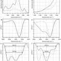For the finite dose case, according to the Organisation for Economic Cooperation and Development (OECD), finite dose experiments are defined by an application of a limited volume of formulation ( $\le$ 10 μl/cm² of a liquid formulation) (OECD 2004a, b). For semisolid and solid formulations, these values range from 1 to 10 mg/cm².

Typical concentration/mass/flux versus time profiles for the infinite, semi-infinite (volume > 10 μl/cm², but with a depletion of the donor which is already perceptive), and finite dose cases are depicted in Fig. 1.1. These theoretical calculations were performed using the DSkin^® software.¹ An aqueous donor/acceptor with a drug diffusion coefficient of 6.33E-5 cm²/s, stratum corneum lipid channel diffusion coefficient of 1.87E-8 cm²/s, and partition coefficient of 6.56 was used for simulations. The initial donor concentration was set to 1 mg/ml, and the donor volume for the semi-infinite dose and finite dose scenario was set as 2 μl and 20 μl, respectively for an area of diffusion of 1.767 cm². A tortious stratum corneum lipid path length of 180 μ m was assumed, which corresponds to a swollen membrane for an in vitro setup (Talreja et al. 2001). Perfect sink conditions of the acceptor compartment are assumed.

Fig. 1.1

Theoretical change of concentration in the donor compartment over time (a), change of mass inside the stratum corneum (b), accumulated mass inside the acceptor compartment (c), and change of stratum corneum outgoing flux (d) for infinite (solid line), semi-infinite (dashed line), and finite dosing (dotted line). Simulations were performed using the DSkin^® software

The chosen values correspond to a model compound of approximately 300 Da with a log K _O/W of 2 in an aqueous vehicle, and model parameters were estimated by DSkin. The concentration-over-time profile depicted in Fig. 1.1a shows the characteristic depletion of the donor for the finite dose case and less pronounced for the semi-infinite case. The barrier mass-over-time curve for an infinite dose setup does reach a plateau as soon as the steady state is reached (Fig. 1.1b). As opposed to this, the mass of the finite dose case decreases after reaching a maximum (Fig. 1.1b). In case of the infinite dose setup, the accumulated mass inside the acceptor compartment reaches the typical straight steady-state line (Fig. 1.1c). This corresponds to a plateau of the flux-over-time profile (Fig. 1.1d). In contrast, the finite dose scenario will reach a theoretical mass plateau in the acceptor compartment if all substance has traveled through the membrane. Obviously, the flux reaches a maximum and subsequently decreases with time. For the simulation of the semi-infinite dose case shown in Fig. 1.1d, the applied volume per area was set slightly higher than the finite dose threshold defined by the OECD. This shows clearly that the assumption of an infinite dose (no significant depletion) does not automatically hold by applying fixed volume-based rules. This is crucial when applying the mathematical concepts presented in the next subsections, since choosing faulty assumptions can lead to serious misinterpretation of experimental data. It has to be kept in mind that even if small volumes of highly concentrated solutions are applied and the permeation is low, the system might behave like an infinite dose case due to the fact that significant donor depletion only occurs at very long experimental time periods in relation to the permeated solute amount in the acceptor compartment.

Investigation of infinite and finite dose experiments typically differ concerning their parameters of interest and application of mathematical concepts (e.g., analytical solutions of the diffusion equation are always tailored to certain boundary and initial conditions). In the next two sections, analytical solutions of the diffusion equation and mathematical concepts for the most typical experimental settings are presented. For an exhaustive compilation of solutions regarding the diffusion equation for various boundary and initial conditions, the reader is kindly referred to the excellent book The Mathematics of Diffusion by J. Crank (Crank 1975).

1.2.1 Dealing with Infinite Dose Skin Permeation

Analysis of infinite dose in vitro skin permeation is typically done by measuring the cumulative amount of substance inside the acceptor compartment over time. For short times, the amount increases exponentially until reaching a steady line (the steady state) with constant flux J _SS (see Fig. 1.2). From a mathematical point of view, a few assumptions must be made to derive an analytical solution for the diffusion equation by defining initial and boundary conditions. In this case, we assume a constant and steady concentration in the donor compartment, perfect sink conditions (zero concentration in the acceptor at all times), and that no compound of interest is located inside the barrier at time $$ t=0 $$

Fig. 1.2

Accumlated mass over time in the acceptor compartment of an infinite dose experiment (solid line) and linear part of the steady-state phase (dashed line). The intersection of the linearized steady-state phase and time axis denotes the lag time

By incorporating these rules for a homogeneous membrane, the absorption curve can be described by an analytical solution of Fick’s second law of diffusion (Scheuplein 1967; Crank 1975), with

$m(t)= A\times K\times l\times {C}_0\left[ K\times l\times t-\frac{1}{6}-\frac{2}{\pi^2}{\displaystyle \sum}_{n=1}^{\infty}\frac{{\left(-1\right)}^n}{n^2} \exp \left(-\frac{D{ n}^2{\pi}^2 t}{l^2}\right)\right]$

(1.11)

Here, A denotes the area of application, K is the partition coefficient between donor and barrier, C ₀ is the concentration of applied formulation in the donor which is assumed not to change significantly during experimental time periods, D is the macroscopic diffusion coefficient, l is the macroscopic thickness of the barrier, and t is the time after application. It is obvious that with t leaning toward infinity (and hence reaching the steadystate), the solution simplifies to the linear part of the steady state (Fig. 1.2), with

$m(t)= A\frac{DK}{l}{C}_0\left( t-\frac{l^2}{6 D}\right)$

(1.12)

From Eq. 1.12, we can examine important parameters when it comes to analysis of infinite dose experiments. The first parameter is the so-called apparent permeability coefficient, k _p _, which is often given in units of cm/h and is defined as

${k}_{\mathrm{p}}=\frac{\mathrm{DK}}{l}$

(1.13)

It is independent of the area of application and initial concentration, and hence a direct parameter for the strength of permeation for a compound through a certain barrier from a specific vehicle under infinite dose and perfect sink conditions. Mathematically, it denotes a normalization of steady-state flux J _SS with

${k}_{\mathrm{p}}=\frac{J_{\mathrm{SS}}}{C_0}$

(1.14)

Such a parameter might heavily depend on experimental conditions. Hence, this has to be kept in mind when comparing parameters (interlaboratory and intralaboratory). Although k _p may be a useful and popular parameter when it comes to examination of permeation experiments, it can be sometimes misleading when comparing the permeation of several compounds (Michaels et al. 1975; Anissimov et al. 2013). The apparent permeability coefficient k _p describes an intrinsic property of a solute to permeate across a specific medium (e.g., the skin) which is independent of the dose but influenced by the applied vehicle. Therefore, comparisons are only possible between compounds which are applied in identical vehicles. In 2006, Sloan et al. introduced a change of paradigm when it comes to explaining experimental data (Sloan et al. 2006). They suggested to use the more expressive parameter J _max which denotes the maximum possible flux of a solute through a barrier for comparing permeability (Eq. 1.15). By using J _max, it is possible to overcome the limitations addressed before

${J}_{\max }={k}_{\mathrm{p}}\times {S}_{\mathrm{v}}= D\times \frac{S_{\mathrm{m}}}{l}$

(1.15)

Here, S _v is the saturated permeant concentration in the vehicle and S _m is the solubility of the solute within the barrier. In other words, by removing the influence of the partition coefficient between the skin and vehicle, J _max should be independent of the vehicle applied. Thus, it describes an intrinsic permeability of a solute in a certain medium, making it an ideal parameter to compare permeability of different solutes. Obviously, this is the case, as long as the vehicle does not affect the transport kinetics in the barrier (Zhang et al. 2011).

In contrast to epidermal k _p which is optimally correlated to the molecular weight and lipophilicity of a compound (Fiserova-Bergerova et al. 1990; Potts and Guy 1992; McKone and Howd 1992), Magnusson et al. (2004) could show that molecular weight is the main determinant when it comes to predicting solute maximum flux.

A further parameter to characterize infinite dose absorption is the so-called lag time t _lag given by

${t}_{\mathrm{lag}}=\frac{l^2}{6 D}$

(1.16)

It is a measure that relates to the time it takes for a compound to travel through the barrier and establish a steady state. A word of caution is necessary concerning the meaning of t _lag. t _lag does not directly represent the time when the steady state is achieved (see Fig. 1.2); however, it can be approximated by multiplying t _lag with 2.7 (Crank showed that steady state is achieved when $\frac{Dt}{l^2}=0.45$ approximately (Crank 1975)).

From a practical point of view, determination of permeability coefficient and lag time can generally be accomplished in two fashions:

1.
The easiest approach utilizes the linearization of the steady state (see Fig. 1.2) which intersects the time axis at t _lag. This can be accomplished graphically by manual interpolation of the last data points that contribute to the steady state or mathematically more soundly by a linear fit (Schäfer-Korting et al. 2008). It is important to mention that the occurrence of physically untenable negative lag times often indicates experimental problems such as donor depletion (Barbero and Frasch 2009) or insufficient sink conditions (Anissimov and Roberts 1999). The permeability coefficient can be determined by dividing the slope of the linear part by the initial concentration C ₀ and application area A or simply by using the two steady-state data points with

${k}_{\mathrm{p}}=\frac{m_{t_1}-{m}_{t_2}}{{\mathrm{AC}}_0\left({t}_1-{t}_2\right)}$

(1.17)
If the slope of the curve decreases after reaching steady state, a general strategy is to employ the steepest part of the curve for evaluation (Buist et al. 2010). The clear advantage is the simplicity in calculations, but several problems arise using this approach that makes it extremely prone to errors – from an experimental and evaluation point of view:
(a)

This approach cannot be applied if the steady state was not clearly reached at the end of the experiment.

(b)

It is often difficult to identify which data points contribute to the steady state and which do not. Often, a frequent sampling and stepwise addition of data points from t _end (last data point) toward t ₀ (first data point) and analyzing the linear interpolations can overcome this problem.

(c)

Using only a limited amount of data points generally ignores information. Carelessly discarding data often yields wrong results and can produce a high variability, depending on which points are chosen for evaluation. This is an obvious but often neglected problem in processing experimental data.
2.

A more sophisticated approach is the use of the mathematical representation of the entire curve (Eq. 1.11). In 2009, Henning et al. performed an in-depth analysis of problems that arise in data evaluation of infinite dose permeation experiments and showed the superiority of this procedure over the manual approach (Henning et al. 2009). A huge advantage is the ability to deliver sound results even if only a partial representation of the steady state is available. Often, the macroscopic thickness of the swollen skin is not exactly known. By defining partition parameter P ₁ and diffusion parameter P ₂ with

${P}_1= K\cdot l$

(1.18)

${P}_2=\frac{D}{l^2}$

(1.19)
and reformulating Eq. 1.11 yields (Díez-Sales et al. 1991; Kubota et al. 1993)

$m(t)= A\cdot {P}_1\cdot {C}_0\cdot \left[{P}_2\cdot t-\frac{1}{6}-\frac{2}{\pi^2}{\displaystyle \sum}_{n=1}^{\infty}\frac{{\left(-1\right)}^n}{n^2} \exp \left(-{P}_2{n}^2{\pi}^2 t\right)\right]$

(1.20)

This reduces the number of unknown parameters. Hence, P ₁ and P ₂ can be easily fitted to experimental data using a nonlinear least squares approach. Permeability and lag time can be subsequently computed by

${k}_{\mathrm{p}}={P}_1\cdot {P}_2$

(1.21)

${t}_{\mathrm{lag}}=\frac{1}{6{P}_2}$

(1.22)

1.2.2 Dealing with Finite Dose Skin Permeation

In contrast to the infinite dose exposure scenario, a typical finite dose absorption profile does not reach a steady state, but builds a mass plateau inside the acceptor compartment at late time points (see Fig. 1.1c). Finite dose experiments also show a characteristic depletion of donor concentration (Fig. 1.1a) and increase in flux until reaching the so-called peak flux J _peak at time t _peak (Fig. 1.3).

Fig. 1.3

Sketch of outgoing flux across the barrier–acceptor interface over time of a finite dose experiment (solid line). The maximum of the curve denotes the peak flux J _max at time to peak flux t _max

As opposed to the infinite dose case, deduction and application of an analytical solution for the description of absorption curves require a more sound mathematical foundation. Based on the theory of heat flow by Carslaw and Jaeger, a description of the flux of the compound leaving the barrier at time t is given by Eq. 1.23 (Carslaw and Jaeger 1959; Cooper and Berner 1985):

$J(t)=2\cdot A\cdot {M}_{\infty}\cdot \beta \cdot \frac{D}{l^2}{\displaystyle \sum}_{i= i}^{\infty}\frac{\alpha_i^2}{ \cos {\alpha}_i\left(\beta +{\beta}^2+{\alpha}_i^2\right)} \exp \left(-\frac{\alpha_i^2\mathrm{Dt}}{l^2}\right),$

(1.23)

with

$\beta = K\frac{l}{h_{\mathrm{v}}},$

(1.24)

and the roots of the transcendal equation, α _i, given by

${\alpha}_i \tan {\alpha}_i=\beta$

(1.25)

Here, ${M}_{\infty }$ denotes the applied mass, and h _v is the height of the formulation in the donor compartment. The remaining parameters keep their meaning as introduced above.

Integrating Eq. 1.23 yields the accumulated mass per area (Kasting 2001) with

$\frac{M(t)}{M_{\infty }}=1-2\beta {\displaystyle \sum}_{i= i}^{\infty}\frac{1}{ \cos {\alpha}_i\left(\beta +{\beta}^2+{\alpha}_i^2\right)} \exp \left(-\frac{\alpha_i^2 Dt}{l^2}\right)$

(1.26)

In comparison to Eq. 1.11 for the infinite dose case, solving Eq. 1.26 requires a more skillful evaluation, since Eq. 1.25 must be solved for arbitrary values of i. A basic strategy to solve the transcendal equation is to use logistic regression to tabulated values of the first roots (see Fig. 1.4). To find further roots a subsequent linear extrapolation from previous roots ( ${\mathrm{root}}_n=2\kern0.5em \times \kern0.5em {\mathrm{root}}_{n-1}\kern0.5em -\kern0.5em {\mathrm{root}}_{n-2}$ ) followed by a refinement step (root-finding with, e.g., Newton’s method) (Kasting 2001) is key. To reduce the number of unknowns, the same approach that worked for the infinite dose case (Eqs. 1.18 and 1.19) can be applied.